How We Process Elevation Data for 30+ Countries

Every time you see contour lines on a MapRiot map, or tilt the view to see 3D terrain, or query our elevation API for a coordinate’s altitude — that data came from somewhere. And getting it from “somewhere” to “rendered on your screen” is one of the more interesting engineering challenges we’ve tackled.

This post walks through our elevation data pipeline: where the raw data comes from, how we process it, and what we learned along the way.

The data sources

There is no single global elevation dataset that’s good enough for detailed outdoor maps. Instead, we use different sources depending on the region:

Europe

For Europe, we primarily use Sonny’s EU DTM data — a unified collection of national lidar and satellite elevation models across European countries, available under CC BY 4.0. Resolution varies by country but is typically around 25m.

The data comes in GeoTIFF files, one per country or region, in various UTM projections. Each Central European country might be in a different UTM zone — Czechia in UTM 33N, France split across 31N and 32N, and so on.

JAXA ALOS AW3D30 (Global)

For countries not covered by European sources, we use the ALOS World 3D 30m dataset from the Japanese Aerospace Exploration Agency. It’s a global satellite-derived DEM at 30m resolution.

JAXA distributes the data in 5-degree tiles. The download process calculates which tiles cover a given country’s bounding box, then fetches them from JAXA’s servers.

National survey data

For countries where we can get it, national survey data beats satellite DEMs. The Czech Republic’s ČÚZK provides elevation data at much finer resolution than any global product. We process these separately, often from national coordinate systems (like the Czech S-JTSK, EPSG:5514) that need reprojection.

The processing pipeline

Regardless of source, the elevation data goes through a similar pipeline. Here’s the flow:

Step 1: Reproject to WGS84

All source data gets reprojected to EPSG:4326 (WGS84) — the coordinate system used by web maps. We use gdalwarp for this:

gdalwarp -t_srs EPSG:4326 \
  -r bilinear \
  -co COMPRESS=ZSTD \
  -co BIGTIFF=YES \
  input.tif output_wgs84.tif

Bilinear resampling is important here. Nearest-neighbor would create staircase artifacts in the elevation data that show up as jagged contour lines. Bilinear interpolation smooths the resampling.

Step 2: Harmonize resolution

Different sources have different native resolutions. When merging multiple countries, we need them all at the same pixel size. We standardize to approximately 25m at the equator (about 0.000256 degrees).

Step 3: Build a virtual mosaic

For hillshading, we merge all country DEMs into a single virtual raster (VRT) using gdalbuildvrt. This lets GDAL treat dozens of separate files as one seamless dataset without actually copying the data:

gdalbuildvrt merged.vrt country1.tif country2.tif country3.tif ...

Step 4a: Generate contours

Contour lines are generated with gdal_contour:

gdal_contour -a elevation -i 10 input.tif contours.shp

This produces contour lines at 10-meter intervals. We then convert these to vector tiles and package them as PMTiles for serving through Martin.

Some countries need special handling. Czech contours from ČÚZK come as pre-computed linestrings in a national projection, so instead of running gdal_contour, we reproject and filter them:

ogr2ogr -t_srs EPSG:4326 -s_srs EPSG:5514 \
  -where "VYSKA % 5 = 0" \
  output.shp input.shp

Step 4b: Generate hillshading tiles

For hillshading, we encode the elevation as RGB values — a technique called terrain-RGB encoding where the red, green, and blue channels encode altitude. The baseline of -10,000m and interval of 0.1m gives sub-meter precision across the full range of Earth’s surface (from the Dead Sea to Everest). The output is packaged as PMTiles at zoom levels 5–12, using WebP compression for efficient storage.

MapLibre GL JS then decodes these RGB values on the client and computes slope shading in real time, simulating a light source from the northwest.

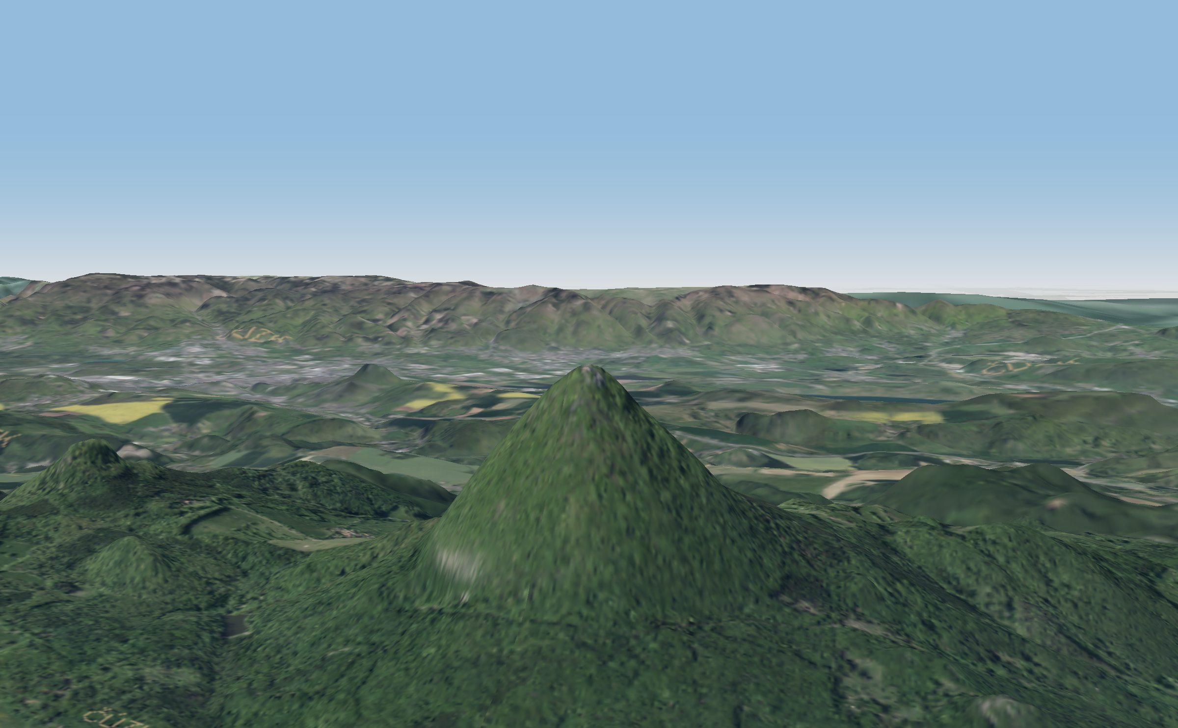
Step 4c: Generate relief tiles

Relief tiles are a pre-rendered raster layer that provides broad terrain shape at low zoom levels (z0–z4). Think of it as a painted relief map — the kind you’d see on a classroom wall. These are generated once and served as static raster tiles.

The numbers

Currently, we process elevation data for over 30 countries. The raw input data (all sources combined) is several hundred gigabytes. The output — contour vector tiles, hillshading raster tiles, and relief tiles — is significantly smaller thanks to tile-level compression and the efficiency of vector formats.

Processing a single country takes anywhere from a few minutes (Luxembourg) to several hours (France, which spans multiple UTM zones and has a lot of terrain).

Elevation API

Beyond tiles, we also expose a simple elevation query API. Given a latitude and longitude, it returns the altitude at that point. This is useful for apps that need to display altitude for a GPS position, compute elevation profiles along a route, or validate that a recorded track’s elevation data makes sense.

The API reads directly from the same DEM data used for tiles, so the accuracy matches what you see on the map.

Lessons learned

Per-country processing is worth the effort. A global pipeline would be simpler to maintain, but the quality difference between European DTM data and JAXA ALOS is visible in the contour lines. National survey data is even better. The extra complexity pays off in map quality.

Compression matters at scale. ZSTD compression on intermediate GeoTIFFs and WebP on output tiles keeps storage manageable. The BIGTIFF flag is essential for any country larger than a few hundred kilometers — standard TIFF has a 4GB file size limit.

Test with edge cases. Coastal areas where land meets sea, international borders where two DEMs meet, and high-altitude regions with sparse data all reveal pipeline bugs that flat terrain won’t find.

The pipeline should be re-runnable. When source elevation data gets updated, we need to reprocess everything. Automation with clear inputs and outputs makes this straightforward.

What’s next

Coverage is expanding steadily — we recently added Oceania and parts of Southeast Asia. We’re also working on incorporating higher-resolution DEMs for popular hiking regions where the difference between 25m and 10m resolution contours is meaningful on the trail. If you need a specific country added, get in touch — we can usually process a new country quickly.

If you’re building an outdoor app and need elevation data, check out our Elevation API docs or browse the map to see the terrain layers in action.